Ensemble Models
The idea behind Ensemble Modeling is that using multiple models together often leads to better predictions than using a single model. The final prediction is based on the combined results of individual models.
Methods of Ensemble Modeling
- Mode/Vote (for Classification): In this method, we create n models, each predicting a category. The final prediction is the mode (most frequently occurring value) among them.
- Averaging (for Regression): For continuous variables, we take the average of predictions from different models to determine the final output.
Pros of Ensemble Modeling
- Captures diverse signals and patterns.
- Reduces incorrect predictions.
- Minimizes overfitting.
- Improves overall model performance.
Cons of Ensemble Modeling
- Increases model complexity.
- Lacks interpretability, which can be a concern in business and finance.
- Requires more computational resources.
Bagging: Random Forest
Bootstrap Sampling is a method of creating different training datasets for models by randomly sampling from the original dataset with replacement.
How Bootstrap Sampling Works?
- Each model receives a random sample from the original dataset.
- Sampling is done with replacement, meaning the same data point can appear multiple times.
- For example, if we have 26 data points:
a, b, c, d, …, z:- We randomly pick one data point and place it in Bootstrap Sample 1.
- This process is repeated 26 times (allowing repetitions) until the sample is complete.
- Similarly, we can create multiple bootstrap samples for different models.
Mathematical Interpretation
For n data points, a total of n! bootstrap samples can be created.
Random Forest: A Special Case of Bagging
Random Forest is an ensemble learning method where multiple decision trees are trained, and their predictions are combined to make the final decision.
How Random Forest Works?
- The base model for Random Forest is a Decision Tree.
- Each tree in the forest makes an independent prediction.
- The final prediction is made by combining the results of all trees (majority vote for classification, average for regression).
Randomness in Random Forest
- Row Sampling (Data Sampling):
- Each tree is trained on a random subset of data (bootstrap sampling).
- Feature Sampling:
- At each split, a random subset of features is considered instead of using all features.
This results in a **two-fold randomness effect**:
✔ Data randomness (at tree level)
✔ Feature randomness (at split level)
Implementation
Firstly, an instance of the bagging-classifier is created under alias BC. Next, we fit the training data in the classifier instance.
from sklearn.ensemble import BaggingClassifier as BC
 classifier = BC()
 classifier.fit(X_train, y_train)
base estimator is a logistic regression model. n-estimators specify number of logistic regression models used to predict final results n-jobs = -1 means all cores of CPU will be used.
from sklearn.linear_model import LogisticRegression as LR

classifier = BC(base_estimator=LR(),
n_estimators=150,
n_jobs=-1,
random_state=42)

classifier.fit(X_train, y_train)
predicted_values = classifier.predict(X_train)
Classification report over test and train data shows a very poor result which is unexpected as bagging algorithm was supposed to be good. This is because we used a linear model as base. And there is no feature transformation over the dataset and hence every logistic regression model is underfit.
from sklearn.metrics import classification_report
 print(classification_report(y_train, predicted_values))
                                            Precision
                                            Recall
                                            F1-Score
                                            Support


                                            0
                                            0.82
                                            0.99
                                            0.90
                                            14234


                                            1
                                            0.75
                                            0.08
                                            0.15
                                            3419


                                            Accuracy
                                            0.82
                                            17653


                                            Macro Avg
                                            0.78
                                            0.54
                                            0.52
                                            17653


                                            Weighted Avg
                                            0.80
                                            0.82
                                            0.75
                                            17653
predicted_values = classifier.predict(X_test)
 print(classification_report(y_test, predicted_values))
                                            Precision
                                            Recall
                                            F1-Score
                                            Support


                                            0
                                            0.82
                                            0.99
                                            0.90
                                            3559


                                            1
                                            0.78
                                            0.09
                                            0.16
                                            855


                                            Accuracy
                                            0.82
                                            4414


                                            Macro Avg
                                            0.80
                                            0.54
                                            0.53
                                            4414


                                            Weighted Avg
                                            0.81
                                            0.82
                                            0.76
                                            4414
Hyper Parameter Tuning
Variation of Train & Test Scores
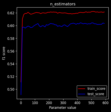
The adjacent graph shows the variation of train score(Red) and test score(blue) with n-estimators over a range of 1 to 600 on steps of 10. It is clear that after some value the score difference almost becomes constant. It is not advisable to use large number of estimators because it will not affect the model performance but increase computational complexity.
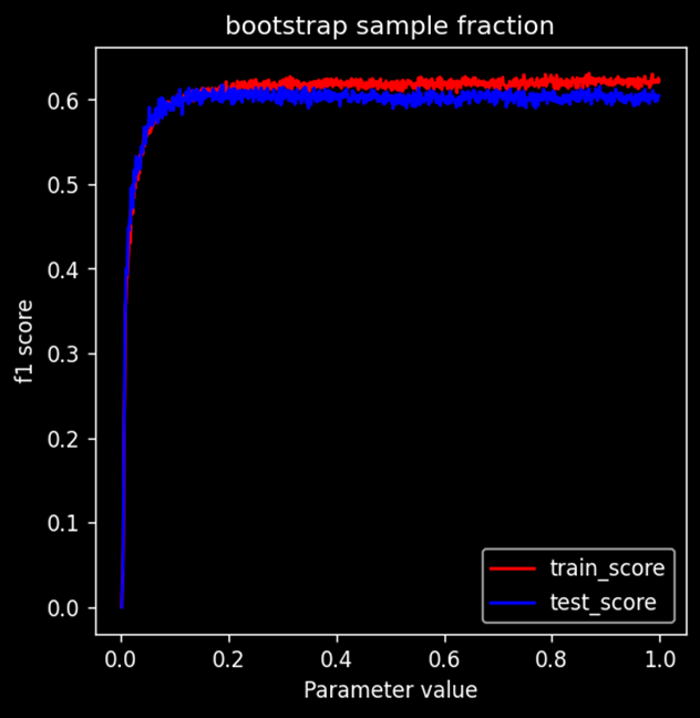
Model Performance variation with dataset fraction
Performance of the model rises sharply and then saturates quickly. From this graph we can conclude that: (Amount of bootstrapped data = amount of original data) this condition is not necessary. Clearly model performance reaches to the max when data provided is less than 0.2 fraction of the original dataset. Giving lesser data will significantly reduce the training time,
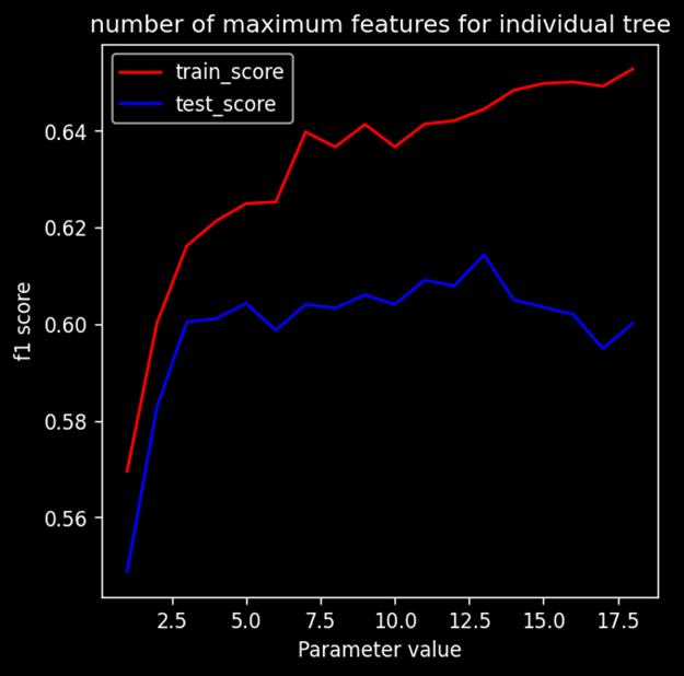
Model Performance vs Number of features
Performance of model initially increases. After a point train score increases whereas test score starts to saturate or decrease, which clearly means model is overfitting after some point Default value of this parameter is set to square root of number of features present in the dataset. Ideal number of max features is close to the default value.