Introduction

Feature Engineering

• Features of a data are the independent variables we use to make predictions.
• To improve predictions, we can:
  • Add external data
  • Use existing data more intelligently
• Feature Engineering is the science of extracting more information from existing data.
• No new data is added, but the data we already have is made more useful with respect to the problem.

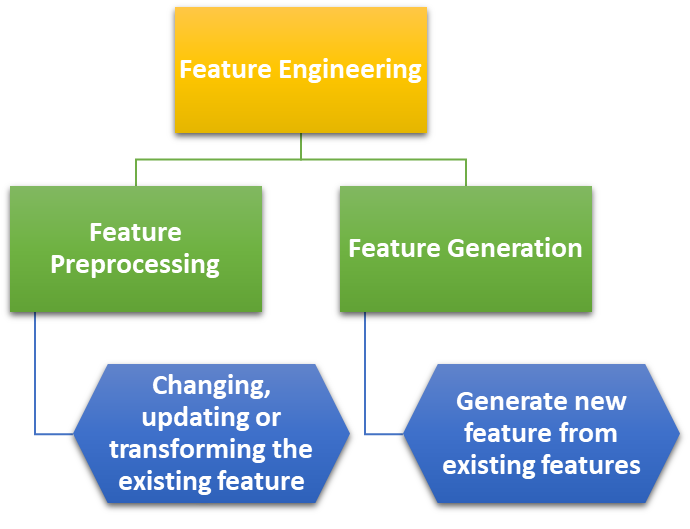
NOTE: Feature generation refers to creating new features from the existing data and not simply transforming the values of existing features.

Transformation Techniques

• Transformation is done to linearize the relationship between target variable and the feature.
• Feature transformation is model specific.
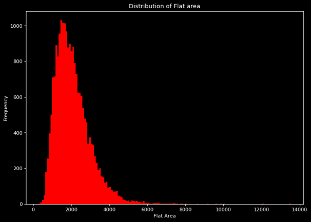
• Transformation can be done to remove skewness in the data curve y vs x,
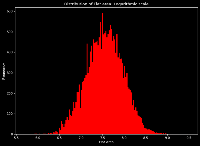
• For right skewed data usually nth root or logarithmic transformation is done.
• For left skewed data usually nth power or exponential transformation is done.

• In our example, in the original raw data set the flat area distribution is right skewed as shown in graph on top
• The result of logarithmic transformation on the graph can be seen in the graph on right.

Categorical Encoding

Categorical encoding is a variable transformation technique for the categorical variables.

DUMMY ENCODING

A separate dummy feature is created for every level present in the categorical column.

LABEL ENCODING

The model detects the relation between the individual categories by itself using the gradient descent. Label encoding is simple to apply. However, in dummy encoding, too many features are added, which results in a lower level of learning.

• Label encoding is used when we want to preserve the existing order among the different categories of the columns.
• This way the dimensionality (number of input variables) remains the same.
• Label encoding is used when the order among different levels is known.

BINNING

Binning is the process of aggregating data points in different categories to reduce redundancy.

This can be implemented on both numerical and categorical columns and also helps in One-Hot Encoding and creating dummy variables.

In binning, we look at the following:

• Binning of categorical variables
• Binning of sparse categories
• Binning of continuous variables

Feature Extraction

• Feature extraction is the process of extracting information from the original features.
• The extracted feature contains the information in simpler form
• This helps in increasing the model performance.

Dimensionality Reduction

Dimensionality Reduction and Feature Selection

High dimensionality can become a problem for prediction modeling. As the number of independent variables increases, visualizing them becomes challenging. Dimensionality reduction is the process of reducing the number of variables from the data to ensure that the reduced data conveys maximum information. To achieve dimensionality reduction, we use the concept of Feature Selection.

Missing Value Ratio (MVR)

The Missing Value Ratio (MVR) is calculated as:

Ratio of missing values = (Number of missing values) / (Total number of observations)

We set a threshold value, say Th, for the missing value ratio (MVR). Based on this, the following actions are taken:

• If MVR ≤ Th, the variable can be estimated.
• If MVR > Th, the variable can be dropped.

It is important to set the threshold very carefully.

Low Variance Removal Technique

In predictive modeling, we often eliminate features with low variance as they do not contribute much to the predictive power of the model. Here, we normalize using a normalizer, not a standard scaler, because a standard scaler would change the variance to 1, making it impossible to compare the variances of different features.

To Remove Categorical Variables:

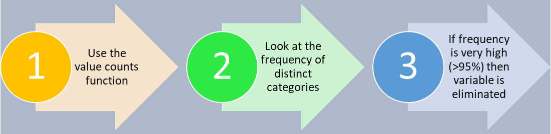
High frequency refers to low variance. In this method, we use the concept of Variance Inflation Factor (VIF) to compute autocorrelation and remove variables accordingly.

Advanced Dimensionality Reduction

There are two methods for advanced dimensionality reduction:

1. Forward selection of features

2. Backward elimination of features

To use these methods, we need an evaluation metric to determine whether any given feature should be selected in the final model or not. The metric used will be Adjusted R².

Adjusted R²

The R² metric has a problem in that it does not consider the number of input variables in the model. The values tend to increase marginally even if the newly added features have zero to minimal importance. To counter this issue, Adjusted R² is introduced. This metric takes into account the number of input features, which reduces the model's performance if the added features do not have a significant effect.

Adjusted R² formula:

\( \text{Adjusted } R^{2} = 1 - \left( \frac{n-1}{n-(k+1)} \right) (1 - R^{2}) \)

• n = sample size or total number of observations
• k = number of input variables
• R² = normal R-squared metric

In the case of simple R², where there are no input variables, k = 0. This turns the entire expression into Adjusted R² = R².

Case I: New feature added contributes significantly to model performance

When the new feature is significant, the increase in R² value will counter the decrement in Adjusted R² due to the increase in k, ultimately leading to an increase in Adjusted R².

Case II: New feature added does not contribute significantly to model performance

If the new feature is insignificant, there is little or no increase in R², but the increase in k will cause the whole expression to decrease.

So, to sum up, Adjusted R² is beneficial when dealing with models that consider multiple features.

Forward Selection

In forward selection, we start with an empty model and add one feature at a time. We evaluate the model at each step and select the feature that gives the best performance. This process is repeated until no further improvement is observed.

• STEP1 : For every independent variable, build a linear regression model individually. Choose the independent variable with the highest adj-R2 score and call it var1.
• STEP2: Repeat the above process by using the var1 as the base independent variable and combining it with every other independent variable to build a regression model. Choose the combination with highest adj-R2.
• STEP3: Repeat the above process until the maximum number of features has been obtained or the adj-R2 is no longer increasing

Backward Selection

In backward selection, we start with all the features and remove one feature at a time. We evaluate the model at each step and remove the feature that gives the best performance. This process is repeated until no further improvement is observed.

Algorithm: BACKWARD ELIMINATION OF FEATURES

• STEP 1 : Build a model with all the independent variables. Adjusted R2 value of this model will be base-line adjusted R2 value.
• STEP 2:
  • Step 2.1 : Drop 1 independent variable at a time
  • Step 2.2 : Build a regression model using all other independent variables
  • Step 2.3 : Calculate the corresponding adjusted – R2.
  • Step 2.4 : Repeat the steps 2.1 – 2.3 for all independent variables
• STEP 3: Subtract the baseline adjusted-R2 from all calculated adjusted-R2 values and record the difference.
• STEP 4: Make the maximum difference value as the new baseline adjusted-R2 and permanently drop the independent variable corresponding to it.
• STEP 5: Repeat the process for the required number of times, which is equal to the number of variables we want to be left with after the completion of backward-elimination-of-features-algorithm.

On performing backward elimination on our linear regression model, we also keep track of adjusted R2 every time we remove a feature. The graph below shows the remaining features vs adjusted R2 at each iteration when we eliminated a feature.

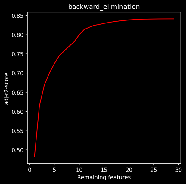
The blue mark is such that if we want to keep the minimum number of features while retaining model performance as much as possible. On the other hand, the green dot represents such a point after which adjusted R2 almost flattens out. So, at this point, we can maximize the model performance and remove only the insignificant variables without harming the adjusted R2 score.

QUESTION: Why do we need two methods that do almost the same thing?

Adjusted R2 has a major drawback that it is computationally expensive. Suppose we have N number of features and it is evident that in every step, one feature is removed from consideration. The total number of models to be created iteration-wise will be:

N + (N-1) + (N-2) + (N-3) + … + 3 + 2 + 1 = N(N+1)/2 ~ N²

For huge datasets, both techniques can be expensive, so we must set a goal:

• Set model interpretation as a priority and only select a small subset of best features to interpret the model (Forward selection is preferred as it focuses on choosing the best features).
• Or strictly remove the features which negligibly add to the model performance (Backward selection is preferred as it focuses on removing the redundant columns first).

Another improvement that can be made is to set a threshold for adjusted R2 such that after getting incremented to that point, the program will stop.